Distance-regular graph

Graph families defined by their automorphisms
distance-transitive	$\rightarrow$	distance-regular	$\leftarrow$	strongly regular
$\downarrow$
symmetric (arc-transitive)	$\leftarrow$	t-transitive, t ≥ 2
$\downarrow$ _{(if connected)}
vertex- and edge-transitive	$\rightarrow$	edge-transitive and regular	$\rightarrow$	edge-transitive
$\downarrow$		$\downarrow$
vertex-transitive	$\rightarrow$	regular
$\uparrow$
Cayley graph		skew-symmetric		asymmetric

In mathematics, a distance-regular graph is a regular graph such that for any two vertices v and w at distance i the number of vertices adjacent to w and at distance j from v is the same. Every distance-transitive graph is distance-regular. Indeed, distance-regular graphs were introduced as a combinatorial generalization of distance-transitive graphs, having the numerical regularity properties of the latter without necessarily having a large automorphism group.

Alternatively, a distance-regular graph is a graph for which there exist integers b_i,c_i,i=0,...,d such that for any two vertices x,y in G and distance i=d(x,y), there are exactly c_i neighbors of y in G_i-1(x) and b_i neighbors of y in G_i+1(x), where G_i(x) is the set of vertices y of G with d(x,y)=i (Brouwer et al. 1989, p. 434). The array of integers characterizing a distance-regular graph is known as its intersection array.

A distance-regular graph with diameter 2 is strongly regular, and conversely (unless the graph is disconnected).

1 Intersection numbers
2 Distance adjacency matrices
3 Examples
4 Notes
5 References

Intersection numbers

It is usual to use the following notation for a distance-regular graph G. The number of vertices is n. The number of neighbors of w (that is, vertices adjacent to w) whose distance from v is i, i + 1, and i − 1 is denoted by a_i, b_i, and c_i, respectively; these are the intersection numbers of G. Obviously, a₀ = 0, c₀ = 0, and b₀ equals k, the degree of any vertex. If G has finite diameter, then d denotes the diameter and we have b_d = 0. Also we have that a_i+b_i+c_i= k

The numbers a_i, b_i, and c_i are often displayed in a three-line array

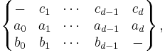
$\left\{\begin{matrix} - & c_1 & \cdots & c_{d-1} & c_d \\ a_0 & a_1 & \cdots & a_{d-1} & a_d \\ b_0 & b_1 & \cdots & b_{d-1} & - \end{matrix}\right\},$

called the intersection array of G. They may also be formed into a tridiagonal matrix

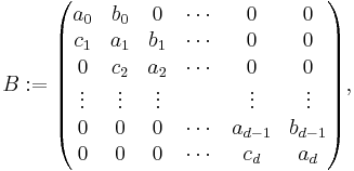
$B:= \begin{pmatrix} a_0 & b_0 & 0 & \cdots & 0 & 0 \\ c_1 & a_1 & b_1 & \cdots & 0 & 0 \\ 0 & c_2 & a_2 & \cdots & 0 & 0 \\ \vdots & \vdots & \vdots & & \vdots & \vdots \\ 0 & 0 & 0 & \cdots & a_{d-1} & b_{d-1} \\ 0 & 0 & 0 & \cdots & c_d & a_d \end{pmatrix} ,$

called the intersection matrix.

Distance adjacency matrices

Suppose G is a connected distance-regular graph. For each distance i = 1, ..., d, we can form a graph G_i in which vertices are adjacent if their distance in G equals i. Let A_i be the adjacency matrix of G_i. For instance, A₁ is the adjacency matrix A of G. Also, let A₀ = I, the identity matrix. This gives us d + 1 matrices A₀, A₁, ..., A_d, called the distance matrices of G. Their sum is the matrix J in which every entry is 1. There is an important product formula:

$A A_i = a_i A_i %2B b_i A_{i%2B1} %2B c_i A_{i-1} .$

From this formula it follows that each A_i is a polynomial function of A, of degree i, and that A satisfies a polynomial of degree d + 1. Furthermore, A has exactly d + 1 distinct eigenvalues, namely the eigenvalues of the intersection matrix B,of which the largest is k, the degree.

The distance matrices span a vector subspace of the vector space of all n × n real matrices. It is a remarkable fact that the product A_i A_j of any two distance matrices is a linear combination of the distance matrices:

$A_i A_j = \sum_{k=0}^d p_{ij}^k A_k .$

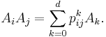
This means that the distance matrices generate an association scheme. The theory of association schemes is central to the study of distance-regular graphs. For instance, the fact that A_i is a polynomial function of A is a fact about association schemes.

Examples

Complete graphs are distance-regular with diameter 1 and degree v−1.
Cycles C_2d+1 of odd length are distance-regular with k = 2 and diameter d. The intersection numbers a_i = 0, b_i = 1, and c_i = 1, except for the usual special cases (see above) and c_d = 2.
All Moore graphs, in particular the Petersen graph and the Hoffman-Singleton graph, are distance-regular.
Strongly regular graphs are distance-regular.
The odd graphs are distance-regular.

Notes

References

A.E. Brouwer, A.M. Cohen, and A. Neumaier (1989), Distance Regular Graphs. Berlin, New York: Springer-Verlag. ISBN 3-540-50619-5, ISBN 0-387-50619-5
Godsil, C. D. (1993). Algebraic combinatorics. Chapman and Hall Mathematics Series. New York: Chapman and Hall. pp. xvi+362. ISBN 0-412-04131-6. MR 1220704.